tharwan.de

Some Words About Physics, Python And The World In General

How we used prefect and MLflow for easy grid searches

At e2m we are currently establishing how we are handling the machine learning model lifecycle. Most of our needs cover time series forecasting in the energy domain. In detail this can cover various things, from market prices, spreads between markets to energy demands or production of individual customers.

There are a number of frameworks out there or in development that help with the modeling itself. But even without these we had reasonable success in the past with using more basic ML frameworks like scikit learn or keras which aren't specialized to time series forecasting .

The much bigger chellange, as is often the case, is of course the operationalisation and maintainance of models. After falling into the trap of trying to develop our own system, we took some time to look around what is "on offer".

In the end, after reviewing several commercial offerings (AzureML, Neptune, Weighs and Biases) as well as open source self-hosted ones (CLearML, MLflow) we felt a little bit lost about what is offered at what price point and what our actual requirements were. And since the best way to discover unknwon requirements is often to just dive into the topic we used OpenMLOps as a starting point (this was helped by our existing usage of prefect as a workflow engine).

And so far we are very happy with our initial expericence of running a setup very similar to OpenMLOps with the biggest difference that we channel all code through a build pipeline. The pipeline effectively does two things, based in the commit message it builds a specified part of the project, packages it in a docker container and registers all related flows in a prefect project. And, again if specified in the commit message, can also trigger a run of a specific flow. (Overall very similar to the apporach descibed here)

This accomplished two things: 1. every developer can schedule a training run without even leaving his IDE on a cluster 2. every run can be traced back to code commited in the central repo

I think it does not make much sense to share too many of the specifics of how we implemented this, since they will either be very close to existing things or differ too much because of different established tools (e.g. wheater you are using Github or Azure DevOps).

However there is one workflow around gridsearch, that utilized existing packages with minimal overhead to produce a very nice workflow we have not seen shared anywhere else so it is probably worth sharing.

Grid Search

With all the available frameworks that help modelling, the task for Data-Scientist becomes much less to programm models itself but rather to quickly find which model and hyper-parameters (e.g. the parameters that define the model) have the best forecasting performance. Again there are frameworks to help this, however we found that with no clear winner in the race for a framework of time series models, we would rather keep it generalized. And as it turns out prefect and sklearn (and Kubernetes) can be combined in rather powerful ways to help.

ParameterGridTask

To quickly start grid searches for existing training tasks we defined a ParameterGridTask that can be used to easily create a parameter search grid.

from sklearn.model_selection import ParameterGrid
from prefect import Flow, Parameter, Task, task, unmapped
from typing import Optional, Callable
import inspect

class PrefectParameterGrid(Parameter):
    def run(self):
        grid = super().run()
        return list(ParameterGrid(grid))


class ParameterGridTask(Task):
    """
    helper class to do grid search.
    """

    def __init__(self, func: Optional[Callable] = None, **kwargs):
        self.func = func
        super().__init__(**kwargs)

    def run(self, **kwargs):
        params = kwargs.pop("grid")
        return self.func(**kwargs, **params)

    def default_parameter(self) -> PrefectParameterGrid:
        """
        Define a Prefect Parameter with the default values of self.func
        :return:
        """
        sig = inspect.signature(self.func)
        func_params_with_default = {
            name: [param.default]
            for name, param in sig.parameters.items()
            if param.empty != param.default
        }
        return PrefectParameterGrid("grid", default=func_params_with_default)

@task
def train(a, b=1, c=2):
    # highly sophisticated training function
    print(a, b, c)
    return a+b+c

# we have to use the function not the Task we created
g_task = ParameterGridTask(func=train.run) 

# this is a placeholder for something like training data
@task
def load_data():
    return 1    

# this generates a parameter which by default has all kwargs from train with their default wrapped in a list
# in this case {"b":[1], "c":[2]}
grid = g_task.default_parameter() 

with Flow("test") as flow:
    # all parameters have to be named, positional parameters are not possible, but this is good practice anyway
    data = load_data()
    g_task.map(a=unmapped(data), grid=grid)

if __name__ == "__main__":
    flow.run(
        run_on_schedule=False,
        parameters={"grid":{"b":[1, 2], "c":[2, 3]}}
        )
# will print 
# 1 1 2
# 1 1 3
# 1 2 2
# 1 2 3

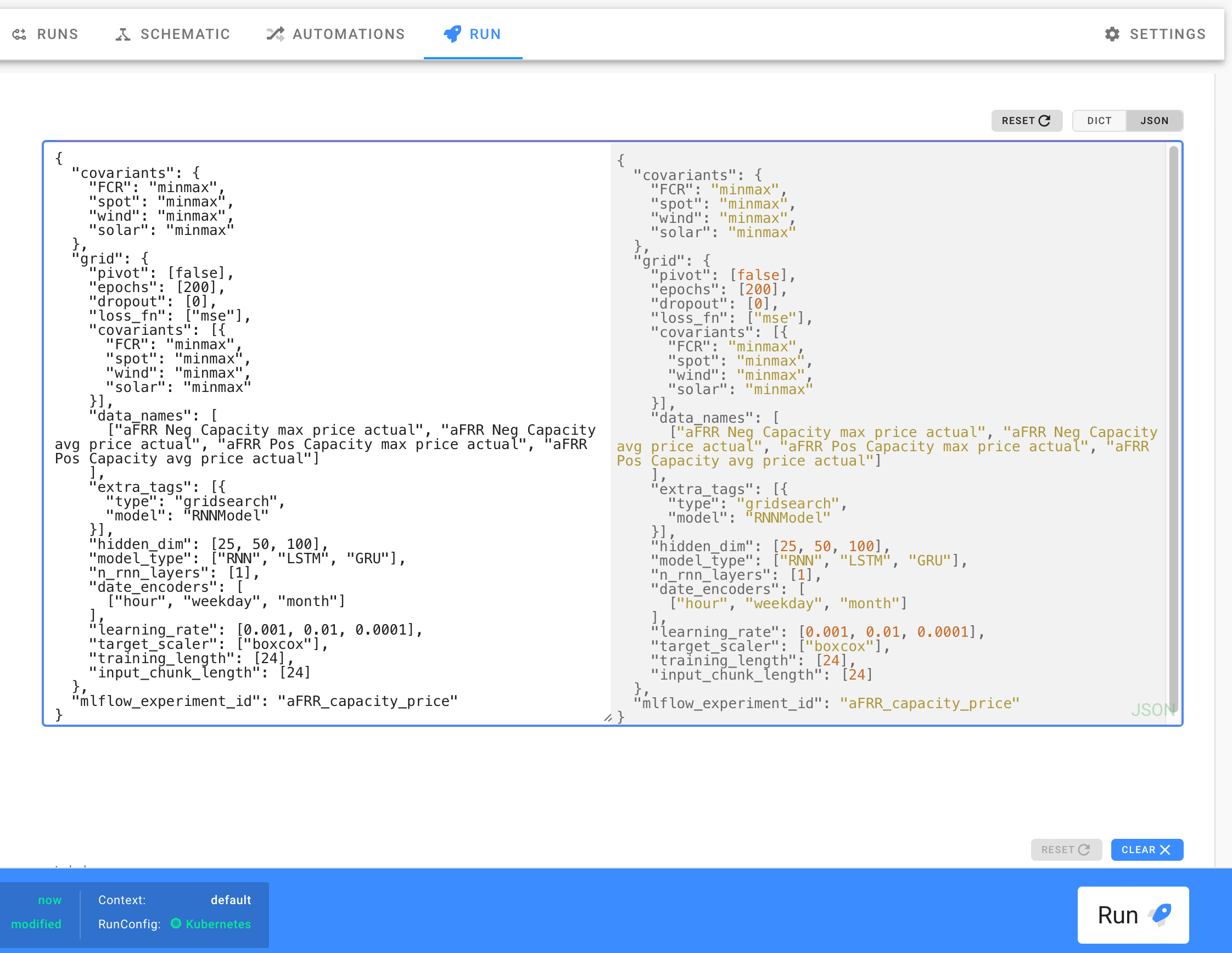
This is will then allow you to quickly define big (be careful) grid searches in the prefect server UI and will automatically pickup any new parameters you add. prefect screenshot

To make this even more powerful one can add a dask executor to a flow, which will distribute the gridsearch among the nodes of a Kubernetes cluster. This only takes a few extra lines but feels enormusly powerful:

from prefect.executors import DaskExecutor
from dask_kubernetes import KubeCluster, make_pod_spec
from typing import Union
import prefect

def create_dask_executor(
    minmum_workers: int = 2,
    maximum_workers: int = 6,
    cpu_limit: Union[float, int] = 1,
    memory_limit: str = "3G",
    idle_timeout: str = "180",
    lifetime: str = "30 minutes",
):
    de = DaskExecutor(
        cluster_class=lambda: KubeCluster(
            make_pod_spec(
                image=prefect.context.image,
                memory_limit=memory_limit,
                memory_request=memory_limit,
                cpu_limit=cpu_limit,
                cpu_request=cpu_limit,
                extra_container_config={
                    "env": [
                        {"name": "MLFLOW_TRACKING_URI", "value": "http://mlflow:5000"},
                        {
                            "name": "DASK_DISTRIBUTED__WORKERS__LIFETIME__DURATION",
                            "value": lifetime,
                        },
                        {
                            "name": "DASK_DISTRIBUTED__WORKERS__LIFETIME__STAGGER",
                            "value": "5 minutes",
                        },
                        {
                            "name": "DASK_DISTRIBUTED__WORKERS__LIFETIME__RESTART",
                            "value": "true",
                        },
                    ]
                },
            ),
            idle_timeout=idle_timeout,
        ),
        adapt_kwargs={"minimum": minmum_workers, "maximum": maximum_workers},
    )
    return de

flow.executor = create_dask_executor()

This cluster will automatically pickup the docker image your flow is using and then start multiple dask workers with it. These works will then go ahead and process all the training tasks defined by the grid search.

Caveats

In practice we found this approach very powerfull and mostly seamless. The biggest problem is that dask appears to inhibit a bug with very long running tasks leading to the workers not consuming any more tasks. One workaround for this is to set a lifetime for the workers as in the above example. One only needs to make sure the training run does not exceed the life time of the worker so no tasks can ever finish.

How much storage does the "Energiewende" need?

A lot.

Since storage is one of the central themes when people are talking about the transition to renewable power, you might have been wondering how much storage do we need. And as many question it has no easy answer, except: "it depends.". It is not easy to find some rough estimates on the web. And where I did, there was no methodology attached to understand their validity. Of course, there are scientific studies but their are hard to access and understand. So I set out to do some, simple as possible, analysis myself. You can find the complete calculations here.

Worst case: 25TWh

Let‘s start straight with the big numbers. Of course, without a reference almost nobody knows if 25TWh is big or not. So lets put them into perspective. Germany currently has about 30 pumped hydro reservoirs. Together they add up to 0.0377 TWh of storage. Which gives us a first glimpse of how much 25TWh are, Germany would need 650x as many pumped hydro installations as it currently has.

Everybody is talking about battery storage these days. So how would li-ion batteries do? Let‘s see: the Tesla Model S is available with 0.1 MWh of storage. This means we would need about 250,000,000 Model S batteries. For comparison there are currently about 43,000,000 cars Germany.

But battery production is picking up quickly around the world. So how long would it take to produce as many as we need? With current battery production output, 880 years. With the estimated output for 2020 only about 140 years. Even if production doubles three more times this is still almost 20 years for Germany‘s storage alone.

Why would we need so much?

The "worst case" would be if we would scale up Germany's current production from wind and solar so that it would just about meet the yearly power consumption. There is no exchange though the power grid with other countries. In this case one would need to store every single kWh that is not used right away to provide for the times when not enough wind is blowing or sun is shining. This would look like the following (data with 15 minute resolution):

2016

We notice two important things in here:

  1. storage fills up during the summer, and is almost drained during autumn
  2. the level in the storage is the same in the beginning and the end of the year

While the second thing is just part of the methodology and you can read more about it in the detailed version of this article, the first one is worth discussing. If we look in detail at the October-November time frame, we can see how there is almost constant underproduction for 4 weeks:

Nov

Therefore these four weeks have a big influence on the overall storage need. Yet we can also see, that production is not zero during these weeks. Therefore if we were to scale up production capacities so that we would produce even more power than we actually need, we would most likely save on storage. It is also important to point out that if we relax our assumption of a 100% renewable system, the storage need can be dramatically decreased by filling the gap during these 4 weeks with fossil fuels.

Production over-capacities will save on storage

This is indeed the case. The first thing we have to realize however is, how far away Germany still is from producing enough electric power from renewables during one year and consequently even further from having over-production. To collect enough power with renewables to fulfill the yearly consumption Germany would need to upscale its current installation by a factor of 4. So 4 times as many solar installations and 4 times as many wind turbines assuming no big changes in efficiency. Of course to achieve over-production even more. It is important to not confuse this with the situation that can already happen, where there is a short term over-production from renewables, and for a few hours they produce more than is needed. In the yearly sum they still only contribute about 25%. That is keeping in mind that we are only looking at the electricity needs here, therefore excluding heating and transport to a large extend.

Over

The above graphic shows the effects of overproduction on the storage need. As we can see the need for storage decreases, the more renewables are installed. Furthermore we see the quite massive amounts of energy that would be overproduced during the course of the year. It needs to be pointed out that this analysis is done in the most simple way, so it does not take into consideration physical constraints about how renewables could be upscaled locally or if their power can be transported with the power grid to where it is needed. But again, the purpose of this exercise is just to get some rough idea about the size of the problem.

So if Germany would manage to produce about 100TWh more than it really needs, the storage would reduce to only 6TWh. While this is still a massive storage (about 60,000,000 Tesla Model S batteries or 35 years of world battery output in 2020) it is only a quarter of the worst case estimate. The interesting thing about this scenario of course is the fact that if essentially produces "free energy".

The case for the smart appliances

However before we dream of what to do with this free energy, there is one more thing that can can be estimated: how much can smart appliances contribute to reduce the storage need. For example if we would use our dishwasher in those minutes when the sun is shining or heat our water when the wind is blowing. For this we assume that the smart appliances will follow the availability of renewable power perfectly, in other words they shift their power usage to not consume during times of low wind and solar availability and vice versa. To simulate this, we can just aggregate our data on a daily basis, so instead of looking at an hourly mismatch between production and consumption we just look at the daily mismatch. So we implicitly assume almost perfect management of the flexible demand (like a smart dishwasher or storage heating). If we then compare the storage need for these daily aggregated data to the previous results, we see how much smart appliances and demand response could save on storage in the best case.

Smart

The above graph shows not only the numbers for daily aggregation but also for weeks and month. The important take away however is the following:

It might be possible that flexible demand will play a bigger role during the transition period, where storage is very rare, but overall its role is limited.

Takeaways

Even though li-ion batteries have come a long way, the energy transition will most likely need other means of storage to become reality.

How much storage does the "Energiewende" need? Roughly?

To get some rought estimates we will at first decide to ignore a few things outright:

  1. that Germany is not alone but part of a European wide grid
  2. Sectorcoupling, i.e. that you can store energy in form of heat, or switch your heating between electric power and burning fossile fuels directly

There are much more sophisticated tools which include these like: PyPSA

Our data source is transparency.entsoe.eu (be sure to select country not bidding zone which is the default) where you can download the data once you created an account. We use the data for load and production for all of 2016. The data comes in 15min time resolution. This Jupyter notebook can also be accessed here.

In [1]:
%matplotlib notebook
import numpy as np
import pandas
import matplotlib.pylab as plt
import datetime
import warnings
In [2]:
#setup a date parser so we can aggregate the data later
dateparse = lambda x: pandas.datetime.strptime(x[:16], '%d.%m.%Y %H:%M')  

#import data with pandas
load = pandas.read_csv("Total Load - Day Ahead - Actual_201601010000-201701010000.csv",
                       parse_dates=[0],date_parser=dateparse,index_col=0)
generation = pandas.read_csv("Actual Generation per Production Type_201601010000-201701010000.csv",
                       parse_dates=[1],date_parser=dateparse,index_col=1)

We will make another assumption concerning power from biomass. Not only does it appear the growth period for biomass in Germany is over, there are also good reasons to not push it any further. In essence, their efficiency is below those of wind and solar, and its use needs to be limited in order to be sustainable.

We will therefore include the generation from biomass into the load, which we assume stays constant over all calculations, while we will scale the production (e.g. wind and solar) up to different values.

In [3]:
#print(generation.columns)

wind_year = generation.filter(regex="Wind.*Actual Aggregated.*").sum().sum()
solar_year = generation.filter(regex="Solar.*Actual Aggregated.*").sum().sum()
bio_year = generation.filter(regex="Biomass.*Actual Aggregated.*").sum().sum()
other_renew = generation.filter(regex="(Waste|Geothermal|Marine|renewable|Hydro Run|Hydro Water).*Actual Aggregated.*").sum().sum()
fossile = generation.filter(regex="(Fossil|Nuclear).*Actual Aggregated.*").sum().sum()


tmp = np.array([wind_year,solar_year,bio_year,other_renew,fossile])/1E6*0.25
labels = ["wind","solar","bio","other","fossile+nuclear"]
plt.figure(figsize=(6,2))
ax = plt.subplot()
left = 0
for idx in range(len(tmp)):
    plt.barh(0,tmp[idx],1,left,label=labels[idx])
    left += tmp[idx]
plt.legend(loc=7)
plt.tight_layout()
plt.xlim((0,450))
ax.set_yticklabels(())
ax.set_yticks(())
Out[3]:
[]
In [4]:
# next we grab the parts that we acually need
# there are some nans in the data mostly because of winter/summer time changes, 
# we fill all missing values from both sides

prod_15_df = generation["Wind Offshore  - Actual Aggregated [MW]"].fillna(method='ffill')
prod_15_df += generation["Wind Onshore  - Actual Aggregated [MW]"].fillna(method='ffill')
prod_15_df += generation["Solar  - Actual Aggregated [MW]"].fillna(method='ffill')

# we also convert the data to MWh, since we have the average for every 15min we just multiply by 1/4 h, 
# e.g. x MW * 0.25 h -> MWh
prod_15_df *= 0.25
prod_15 = prod_15_df.values


load_15_df = load["Actual Total Load [MW] - Germany (DE)"].fillna(method="ffill")
# the biomass production gets subtracted from the load as we assume it stays constant
load_15_df -= generation["Biomass  - Actual Aggregated [MW]"].fillna(method='ffill')
other_renew = generation.filter(regex="(Waste|Geothermal|renewable|Hydro Run|Hydro Water).*Actual Aggregated.*")
for col in other_renew.columns:
    print(col)
    load_15_df -= generation[col].fillna(method="ffill")
load_15_df *= 0.25
load_15 = load_15_df.values
Geothermal  - Actual Aggregated [MW]
Hydro Run-of-river and poundage  - Actual Aggregated [MW]
Hydro Water Reservoir  - Actual Aggregated [MW]
Other renewable  - Actual Aggregated [MW]
Waste  - Actual Aggregated [MW]

How much do renewables contribute?

The data set also contains data for other renewable energy production, which are quite minor in Germany. The first thing to do now is to scale up the production of solar and wind so that it will match the yearly energy consumption.

In [5]:
scale = np.sum(load_15)/np.sum(prod_15)
print("yearly load {:.2f}TWh\nyear's renewable production {:.2f}TWh".format(np.sum(load_15)/1E6,np.sum(prod_15)/1E6))
print("upscaling factor: {:.2f}".format(scale))
prod_fit = prod_15 * scale
yearly load 423.55TWh
year's renewable production 111.27TWh
upscaling factor: 3.81

As we can see, we need about 4x as many renewables than what is currently installed in Germany, just provide enough electricity as is needed during one year. We more or less already knew that, since renewables only account for 1/4 to 1/5 of Germany electricity supply.

Before we have a look at the data, there is one more thing to point out, as there seems to be a bit of a mismatch between the numbers here and, for example, the data on this wikipedia page or this German one, that all list different number for the overall electricity consumption in 2016.

I assume that the numbers in this data here concern only the electricity which was traded via the spot market, while other data may also contain other long term contracts. Whatever may be the case, for a rough number it should be good.

So let's have a look at the data:

In [6]:
fig = plt.figure(figsize=(8,4))
ax1 = plt.subplot()
x = generation.index
ax1.plot(x,prod_fit/1E3,label="production")
ax1.plot(x,load_15/1E3,label="load")
ax1.set_ylabel("GWh")
plt.legend()
plt.grid()
plt.title("2016")
plt.tight_layout()

As we might expect, we see a very constant and somewhat predictable load curve, while production varies wildly.

In [7]:
fig = plt.figure(figsize=(8,4))
ax1 = plt.subplot()
x = generation.index
start = 1500
stop = start + 14*24*4
ax1.plot(x[start:stop],prod_fit[start:stop]/1E3,label="production")
ax1.plot(x[start:stop],load_15[start:stop]/1E3,label="load")
ax1.set_ylabel("GWh")
plt.legend()
plt.grid()
plt.title("2016")
plt.ylim((0,36))
plt.tight_layout()

If we zoom in on these two weeks in January, we can see one of the major problems to face already. During the first week we have almost constantly too little production, while in the second week we have excess production for most of the time. So we need to store the energy not only for a few hours (from mid day to provide light during the evening, for example), but for at least a full week.

So let's calculate how much we will store or draw from storage. We will ignore any losses at first, just for some very simple approximations. We just calculate the difference between production and consumption at any point in time:

$$D_t = P_t - C_t$$

We can then sum up this difference over time, which will give us the storage level at any point:

$$S_t = \sum_{i=0}^t P_i - C_i$$

Since we set $\sum_T P_t = \sum_T C_t$ we know that $S_t$ will be 0 for $t = T$ or, in other words, we will end with the same level in the storage as we begun. However, we might run below zero during the course of the year. To correct for that we just subtract the minumum point afterwards, as you will see.

In [48]:
diff_15 = prod_fit - load_15  #our D_t
storage_15 = np.cumsum(diff_15)  #S_t

plt.figure(figsize=(8,4))
x = generation.index
ax1 = plt.subplot()
lines = ax1.plot(x,prod_fit/1E3,label="production")
lines += ax1.plot(x,load_15/1E3,label="load")

ax1.set_ylabel("GWh")

ax2 = ax1.twinx()
#lines += ax2.plot(x,(storage_15)/1E6,'k--',label="storage")
lines += ax2.plot(x,(storage_15-min(storage_15))/1E6,'k',label="storage")
ax2.set_ylabel("TWh")
labels = [l.get_label() for l in lines]
plt.legend(lines,labels)
plt.title("2016")

plt.tight_layout()

It is important to note that we changed the scale of the storage axis (from GWh to TWh!), as otherwise we could not see anything.

So let's zoom in again into the two weeks of January.

In [47]:
plt.figure(figsize=(8,4))
x = generation.index
start = 1500
stop = start + 14*24*4

ax1 = plt.subplot()
lines = ax1.plot(x[start:stop],prod_fit[start:stop]/1E3,label="production")
lines += ax1.plot(x[start:stop],load_15[start:stop]/1E3,label="load")

ax1.set_ylabel("GWh")
ax2.set_ylim((0,36))

ax2 = ax1.twinx()
#lines += ax2.plot(x,(storage_15)/1E6,'k--',label="storage")
lines += ax2.plot(x[start:stop],(storage_15[start:stop]-min(storage_15))/1E6,'k',label="storage")
ax2.set_ylabel("TWh")
ax2.set_ylim((0,8))
labels = [l.get_label() for l in lines]
plt.legend(lines,labels,loc=9)
plt.title("2016")

plt.tight_layout()

As we would expect, storage gets drained during the first week and filled up again in the second. You might be wondering if the storage needed would change if we would include the beginning of the next and the end of the last year. Indeed we leave the storage the same way we found, however if the following year would require a higher starting level it would indeed change the outcome. However since we already analyzed a full year and each year is at least somewhat similar due to the seasons, including another week or minth should not change much about the estimation. The data is also available, so the analysis can be done, but for an estimate it‘s not really needed.

But how much storage do we need now?

In [26]:
storage_needed_15 = (np.max(storage_15)-np.min(storage_15))
print("storage needed {:.2f} TWh".format(storage_needed_15/1E6 ))
storage needed 22.98 TWh

Well ok 23 TWh, but how much is that?

Let's see: we can compare it to pumped hydro storage

In [27]:
current_hydro = 37700  #MWh in Germany from Wikipedia
print("current pumped hydro: {} TWh\nupscale factor: {:.0f}".format(current_hydro/1E6,storage_needed_15/current_hydro))
current pumped hydro: 0.0377 TWh
upscale factor: 610

Ok, so we need more than 600x as much hydro as we currently have. So that does not seem like a good strategy.

What about Batteries?

Li-Ion batteries are all the rage these days, so why don‘t we use some of them? Lets see how many we would need.

In [28]:
tesla_model_s = 0.1  #MWh
tesla_power_wall = 0.013 #MWh
tesla_power_pack = 0.2 #MWh
print("{:13,.0f} Model S batteries or\n{:13,.0f} power walls or\n{:13,.0f} power packs.".format(
    storage_needed_15/tesla_model_s,storage_needed_15/tesla_power_wall,storage_needed_15/tesla_power_pack))
  229,833,410 Model S batteries or
1,767,949,310 power walls or
  114,916,705 power packs.

So if we compare this with some of the well known Tesla products that use batteries we still find we a need a lot. In fact there are currently only about 43,000,000 cars in Germany. So even even they would all be Teslas and not used for driving, we would still need 4x as many cars.

Ok, but the production of batteries is picking up quickly around the world. So at least it should not take too long to make the batteries we need?

In [29]:
battery_production_2016 = 28E3 # 28 gigawatt-hours
battery_production_2020 = 174E3 # 174 gigawatt-hours
print("With 2016 output it takes about {:.0f} years of battery production.".format(storage_needed_15/battery_production_2016))
print("With estimated 2020 output {:.0f} years.".format(storage_needed_15/battery_production_2020))
With 2016 output it takes about 821 years of battery production.
With estimated 2020 output 132 years.

That is too long, even if production doubles a few more times it takes at least 20 years and that would be for Germany only. We have too look into the details a bit more.

Why do we even need so much?

In [43]:
plt.figure(figsize=(8,4))
x = generation.index
start = 27600
stop = start + 34*24*4

ax1 = plt.subplot()
lines = ax1.plot(x[start:stop],prod_fit[start:stop]/1E3,label="production")
lines += ax1.plot(x[start:stop],load_15[start:stop]/1E3,label="load")

ax1.set_ylabel("GWh")
ax2.set_ylim((0,36))

ax2 = ax1.twinx()
#lines += ax2.plot(x,(storage_15)/1E6,'k--',label="storage")
lines += ax2.plot(x[start:stop],(storage_15[start:stop]-min(storage_15))/1E6,'k',label="storage (corrected)")
ax2.set_ylabel("TWh")
ax2.set_ylim((0,20))
labels = [l.get_label() for l in lines]
plt.legend(lines,labels)
plt.title("2016")

plt.tight_layout()

If we look at the first plot showing the storage usage during the whole year, we can see how our storage gets filled during the summer months and then drains rapidly during autumn. As we can see in the above figure, from the middle of October till the middle of November we have almost constant under production. So much so that we would have drained almost 3/4 of our storage. These four weeks are the main reason we need so much storage.

How to reduce the storage need?

Nevertheless, we are not underproducing all that much on most of the days. So what we could do is not just build as many renewables as we absolutely need, but just a few more. This will however complicate the storage calculation a bit.

What we have to do now is not just sum up the differences, as this would just fill our storage more and more. Instead we have to work our way backwards thought the year. For each timestep we check how much we over- or underproduced. If we have underproduction we add it to our storage need, since we now that this under production needs to be taken from storage which has to be filled in the days before. Then we look at the next time step which, since we are going backwards, is in fact the one before the current one. If we had over production in this time step, we can subtract it from you storage need until the storage need is 0. If we had underproduction in this timestep too we just add it to the storage need. We also keep track of the storage need for each time step we visit. This way if we need something from the storage in three consecutive days, we will have a very high storage need calculated in the day before that. But we also keep track of the possibility to refill the storage anytime.

In [31]:
def calc_need(diff):
    need = np.zeros_like(diff)
    state = 0
    for idx,d in enumerate(diff[::-1]):  #we iterate in reverse order
        if state + d > 0:
            need[idx] = 0
            state = 0
        else:
            need[idx] = -state - d
            state += d
    return need[::-1]  #and then reverse the result again
In [32]:
over_scale = 4.5
prod_over = prod_15 * over_scale

diff_over = prod_over - load_15
need = calc_need(diff_over)
storage_need = np.max(need)

print("storage needed {:.2f} TWh".format(storage_need/1E6))
storage needed 9.83 TWh

With only a slight overproduction we already decreased the storage need quite dramatically, to about half of what we needed before.

We can also calculate how our storage level would look like at any given point in time and use it to check if our calculations are correct. We just set the maximum level of storage need we calculated by going backwards though the year as our storage capacity, then fill the storage with any over-production and drain it as needed.

Furthermore, with this kind of backtracking, we can also consider the storage losses that would occour from self-discharge of Li-Ion batteries. We just need to consider that our storage need grows every time we move one timestep. It grows since we are moving backwards through the year and we are keeping track of the storage needs. So during one step forward in time, we would loose some energy, which means if we go backwards we need more capacity.

In [33]:
# Li-Ion batteries loose about 2-3% of charge per month of storage
qHour_in_month = 30*24*4
days_in_month = 30

def calc_need(diff,subs,loss_per_month = 1-0.02):
    loss_per_sub = np.exp(np.log(loss_per_month)/subs)
    need = np.zeros_like(diff)
    state = 0
    for idx,d in enumerate(diff[::-1]):
        if state + d > 0:
            need[idx] = 0
            state = 0
        else:
            state /= loss_per_sub
            need[idx] = -state - d
            state += d
    return need[::-1]

def calc_level(diff,subs,loss_per_month = 1-0.02):
    loss_per_sub = np.exp(np.log(loss_per_month)/subs)
    batt = np.zeros_like(diff)
    tmp = -np.min(np.cumsum(diff))*1.1  # 1.1 as safety margin
    for idx,d in enumerate(diff):
        tmp = min((storage_need,tmp*loss_per_sub+d))
        batt[idx] = tmp
    return batt
In [34]:
need = calc_need(diff_over,qHour_in_month)
storage_need = np.max(need)
level = calc_level(diff_over,qHour_in_month)

x = generation.index
plt.figure(figsize=(8,4))
plt.plot(x,level/1E6,label="level")
plt.plot(x,need/1E6,label="need")
plt.ylabel("TWh")
plt.grid()
plt.legend()
plt.tight_layout()

As we can see, the storage will indeed be fully used during the critical time in November. We also exit the year with an almost full storage.

Let‘s see how much over-capacity reduces storage need

In the next figure we will compare the needed storage depending on how much more renewable capacity we installed then we would absolutly need. We can also use this to see the influence of the storage losses we introduced.

In [36]:
test_values = np.arange(3.9,10,0.3)
storage_need_array = np.zeros_like(test_values)
storage_need_array_nL = np.zeros_like(test_values)
over_production = np.zeros_like(test_values)
over_TWh = np.zeros_like(test_values)

for idx,over_scale in enumerate(test_values):
    prod_over = prod_15 * over_scale
    diff_over = prod_over - load_15

    over_production[idx] = np.sum(diff_over) / np.sum(prod_fit)
    over_TWh[idx] = np.sum(prod_over) - np.sum(load_15)
    #print(np.sum(prod_over)/1E6-np.sum(load_15)/1E6)
    need = calc_need(diff_over,qHour_in_month)
    storage_need_array[idx] = np.max(need)

    need = calc_need(diff_over,qHour_in_month,1)
    storage_need_array_nL[idx] = np.max(need)


plt.figure(figsize=(5,4))
ax1 = plt.subplot()
ax1.plot(over_production*100,storage_need_array/1E6,'*-',label="with loss")
ax2 = ax1.twiny()
ax1.plot(over_production*100,storage_need_array_nL/1E6,'*-',label="without loss")

all_prod = np.sum(prod_fit)
tmp = np.array(ax1.get_xticks())/100*all_prod


ax2.set_xlim(ax1.get_xlim())
ax2.set_xticklabels(["{:.0f}".format(x) for x in tmp/1E6])
plt.ylim((0,25))
ax1.set_ylabel("storage needed (TWh)")
ax2.set_xlabel("overproduction (TWh)")
ax1.set_xlabel("overproduction (%)")
ax1.legend()
Out[36]:
<matplotlib.legend.Legend at 0x1104dff60>

These results actully tells us two things:

  1. Losses only play a big role in the initial scenario, where we produce just as much as we need and, therefore, store energy for longer times;
  2. We have an almost exponential decrease in storage need, which then becomes more linear above 20% over production.

Make no mistake, it might look like an easy option to simply build 5x more renewables instad of just 4x times as much. However, the availability of too much power over long stretches of time might have massive consequences. It might "just" drive up consumption, as it will be cheaper during that time, or it might change the whole energy system. Electricity has been comparably cheap for a long time now, but if the capacity of installed renewables delivers more then we need over long stretches of time, energy will essentially be for free. There still costs attatched to maintainance and investments need to be repaid, but these costs are no longer related to the amount of power produced.

Additionally, once there is "free energy" other less efficient storage methods like power to gas become much more attractive. However, it might be that a lot of this energy might also be exported to other European countries, depending on the weather conditions there.

Either way, there is at least one more question we can explore with this data set. I will at first formulate the question in a more boring way, however, we can interpret the results in a much more exciting manner later on.

So the boring question is:

What is the role of time scales?

Does it matter if we look at the problem of storage on a sub-hourly level or with a montly resolution?

To explore this we will group the data by hours, days, weeks and months, to see how this changes the amount of storage that we need. So instead of looking at the data with 15 minute resolution, we sum it up to 60 minutes, 24 hours and so on.

In [39]:
def storage_time_group(scale):
    storage_need_ts = []

    prod_over = prod_15 * scale
    diff_over = prod_over - load_15

    need = calc_need(diff_over,30*24*4)
    storage_need_ts.append(np.max(need))
    over_production = np.sum(diff_over) / np.sum(prod_over)

    prod_60 = prod_15_df.groupby(pandas.TimeGrouper(freq="h")).sum().values
    load_60 = load_15_df.groupby(pandas.TimeGrouper(freq="h")).sum().values
    prod_60 *= scale
    diff_60 = prod_60 - load_60

    need = calc_need(diff_60,30*24)
    storage_need_ts.append(np.max(need))

    prod_day = prod_15_df.groupby(pandas.TimeGrouper(freq="D")).sum().values
    load_day = load_15_df.groupby(pandas.TimeGrouper(freq="D")).sum().values
    prod_day *= scale
    diff_day = prod_day - load_day

    need = calc_need(diff_day,30)
    storage_need_ts.append(np.max(need))

    prod_week = prod_15_df.groupby(pandas.TimeGrouper(freq="w")).sum().values
    load_week = load_15_df.groupby(pandas.TimeGrouper(freq="w")).sum().values
    prod_week *= scale
    diff_week = prod_week - load_week

    need = calc_need(diff_week,4)
    storage_need_ts.append(np.max(need))

    prod_month = prod_15_df.groupby(pandas.TimeGrouper(freq="M")).sum().values
    load_month = load_15_df.groupby(pandas.TimeGrouper(freq="M")).sum().values
    prod_month *= scale
    diff_month = prod_month - load_month

    need = calc_need(diff_month,1)
    storage_need_ts.append(np.max(need))

    return over_production,np.array(storage_need_ts)

plt.figure()
storage_time_dict = {}
for scale in np.arange(3.9,7,0.5):
    over_prod,res = storage_time_group(scale)
    storage_time_dict[over_prod] = res
    plt.plot(range(len(res)),res/1E6,'*--',label="{:.0f}% overproduction".format(over_prod*100))

plt.xticks(range(len(res)), ["15 min","60 min","day","week","month"])
plt.ylim((0,25))
plt.grid()
plt.ylabel("TWh")
plt.tight_layout()
plt.legend(loc=0)
Out[39]:
<matplotlib.legend.Legend at 0x10f314eb8>

What we see in these results is nothing too surprising, if we look at more coarse time scales, we would need less storage. If we only look at the monthly data, e.g. how much we have produced and consumed during whole Janurary, we might not see that we have a lack of production during the first week and over production during the second. On a first look the only intersting outcome is that there is very little change between quarterhourly, hourly and daily grouping of the data, which tells us we should work with at least daily time resolution.

How much "storage" can we get from smart appliances?

However we can also interpret this data differently. Take for example the daily aggregated data. In this data we do not look anymore if there was enough production for the peak hours in the morning or evening, we just check if there was as much production as consumption for the whole day. This way of ignoring the daily peaks can be thought of as and ideal form of demand response. Since we consume all of the days' energy whenever it is available, consumption perfectly follows production, which is nothing more than demand response at its core.

Therefore, this data can also answer the question of how much the "smart dishwasher" can help us reduce the need for storage by adjusting the time when it cleans the dishes. So let's rearrange things so that we can better see these changes. For that, we will plot just the change of storage need in comparison to the base scenario of 15 minutes resolution:

In [40]:
plt.figure(figsize=(8,4))
best = np.zeros(4)

with np.errstate(divide='ignore'):
    for op,res in storage_time_dict.items():
        plt.subplot(121)
        plt.plot(range(len(res)-1),(res[1:]-res[0])/1E6,'*--',label="{:.0f}% overproduction".format(op*100))
        plt.subplot(122)
        plt.plot(range(len(res)-2),(res[1:-1]-res[0])/res[1:-1]*100,'*--',label="{:.0f}% overproduction".format(op*100))
        best = np.minimum(best,(res[1:]-res[0])/res[1:])

plt.subplot(121)
plt.xticks(range(len(res)-1), ["60 min","day","week","month"])
plt.grid()
plt.ylabel("TWh")

plt.legend(loc=0)

plt.subplot(122)
plt.xticks(range(len(res)-2), ["60 min","day","week"])
plt.grid()
plt.ylabel("%")

plt.tight_layout()
print("biggest decrease for:\ndayliy load shift: {:.2f}%\nweekly load shift: {:.2f}%".format(best[1]*100,best[2]*100) )
biggest decrease for:
dayliy load shift: -19.35%
weekly load shift: -66.81%

Looking at the data this way might be a little big discouraging at first. If we assume a smart applicance can only shift load within a day or less, the resulting storage decreases are very little, saving about half a TWh of storage. Nevertheless, with current technology storage is expensive and not needing 500GWh would mean many pumped hydro stations would not need to be built. In case of very high overproduction, demand response might even reduce the storage need by 10 to 20%.

Conclusions

  • For powering Germany with Wind, Solar and Biomass we need at least 5TWh of storage.
  • To reduce storage need significant over-production is needed
  • The use of li-ion batteries to power the whole system seems very questionable
  • The role of demand response is very limited

This whole notebook can be downloaded here.

 page 1 / 9  older